In recent years, diffusion models have emerged as the state-of-the-art frameworks for continuous data generation, enabling the synthesis of high-quality data, such as images, audio and video [7, 8]. Their strong generation performance, training stability and flexibility motivated their extension to discrete data, including texts, graphs, or molecule sequences [2, 5, 6]. This blog post is a pedagogical introduction to the adaptation of diffusion models for discrete data.

As continuous-space diffusion models have been developed into two major branches, namely the variational [10, 11] and the score-based ones [9, 12], we present discrete diffusion through these two formalisms. We first introduce variational discrete diffusion; the reader already familiar with this technique can jump directly to the score-based perspective. Finally, in the last section, we first show how these two different viewpoints are in fact equivalent from both the training and sampling perspectives, then show the equivalence of discrete diffusion and discrete flow matching.

In this blog post, we deal with discrete data: the space on which the probability distributions are defined is $\mathcal{S} := \mathcal{V}^S$, namely the space of sequences of length $S \in \mathbb{N}$ over a given vocabulary $\mathcal{V}$. A sequence $\mathbf{x}$ in $\mathcal{S}$ is denoted as $\mathbf{x} = x^1 \dots x^S$, the $x^i$‘s being called tokens. In the vocabulary, we add a special token: the mask token, denoted as $m$. The reader interested to have a more complete introduction on discrete data modelling is referred to the blog post on discrete flow matching.

Variational discrete diffusion

Continuous-space diffusion models learn to generate data, e.g. images, by reversing a forward process that gradually corrupts data into pure noise through the addition of Gaussian noise. In discrete diffusion, an analogous approach generates sequences by reversing a masking process that progressively replaces tokens with a mask token.

Forward process

We first consider the forward process: it starts from a clean sequence $\mathbf{x}_0$, and progressively replaces each token by the mask token, transforming the sequence into $\mathbf{x}_T = mm...m$. Because each token is masked independently, the forward process factorizes over tokens, and we restrict to the case of a single token transitioning from $x_0^i$ to $m$ in the following.

In continuous Denoising Diffusion Probabilistic Models (DDPM), we start by defining a noising process over $T$ steps, where each step slightly corrupts the signal by adding Gaussian noise:

$$\begin{equation} \htmlData{equation-label=eq:ddpm-step}{\htmlId{eq:ddpm-step}{}} x_t = \sqrt{1 - \beta_t}\, x_{t-1} + \sqrt{\beta_t}\,\varepsilon, \qquad \varepsilon \sim \mathcal{N}(0, I) \end{equation}$$

where $\beta_t \in [0,1]$ controls the amount of noise injected at step $t \in \{1,\ldots,T\}$. In discrete space diffusion, at each step, a token either survives unchanged with probability $1 - \beta_t$, or is irreversibly replaced by the mask token $m$ with probability $\beta_t$:

$$\begin{equation} \htmlData{equation-label=eq:mdm-step}{\htmlId{eq:mdm-step}{}} x_t = \begin{cases} x_{t-1}, & \text{with probability } 1 - \beta_t \\ m, & \text{with probability } \beta_t \end{cases} \end{equation}$$

From Eq. (?), we can infer the law of $x_t$ given its starting value $x_0$, without simulating the full chain:

$$q(x_t = x_0 | x_0) = \prod_{i=1}^{t} (1-\beta_i) =: \alpha_t$$

and we can interpret $\alpha_t$ as the probability that a token has survived up to step $t$, i.e. $x_t$ is still $x_0$ and was not replaced by $m$.

Proof

$$\begin{align} q(x_t = x_0 | x_0) &= \underbrace{q(x_t = x_0 | x_{t-1} = x_0, x_0)}_{ \substack{=\,q(x_t = x_0 | x_{t-1} = x_0)\text{ by the Markov property}}}\, q(x_{t-1} = x_0 | x_0) \\ &= (1-\beta_t)\, q(x_{t-1} = x_0 | x_0) \\ &= \prod_{i=1}^{t} (1-\beta_i) \qquad \text{by recursion} \end{align}$$

As expected, the schedule $\alpha_t$ decreases in $t$: as the step index $t$ increases, the probability of a token remaining unmasked decreases. You can observe this trend in Figure 1 when selecting “Show N trajectories”. It turns out that we can then compute the transition probabilities between any two steps $s < t$ as follows:

$$\begin{equation} \htmlData{equation-label=eq:forward-transition}{\htmlId{eq:forward-transition}{}} x_t \mid x_s = \begin{cases} x_s, & \text{with probability } \frac{\alpha_t}{\alpha_s} \\ m, & \text{with probability } 1 - \frac{\alpha_t}{\alpha_s} \end{cases} \end{equation}$$

Proof

By the Markov property $q(x_t | x_s, x_0) = q(x_t | x_s)$, the marginal $q(x_t | x_0)$ factorizes through any intermediate step $s$:

$$\begin{equation} \htmlData{equation-label=eq:marginal-recursion}{\htmlId{eq:marginal-recursion}{}} q(x_t | x_0) = \sum_{x_s} q(x_t | x_s)\, q(x_s | x_0) \end{equation}$$

Using $q(x_s | x_0) = \alpha_s\, \mathbb{I}(x_s = x_0) + (1 - \alpha_s)\, \mathbb{I}(x_s = m)$, the sum simplifies to:

$$\begin{equation} \htmlData{equation-label=eq:marginal-split}{\htmlId{eq:marginal-split}{}} q(x_t | x_0) = \alpha_s\, q(x_t | x_s = x_0) + (1 - \alpha_s)\, q(x_t | x_s = m) \end{equation}$$

Since masking is irreversible, $q(x_t | x_s = m) = \mathbb{I}(x_t = m)$. Writing $q(x_t | x_s = x_0) = a\, \mathbb{I}(x_t = x_0) + (1 - a)\, \mathbb{I}(x_t = m)$, for $x_t = x_0$, Eq. (?) becomes: $\alpha_t = \alpha_s \cdot a$, so $a = \dfrac{\alpha_t}{\alpha_s}$

Therefore, for an unmasked token $x_s \neq m$ (since the probabilities sum to 1):

$$\begin{equation} \htmlData{equation-label=eq:masked-transition}{\htmlId{eq:masked-transition}{}} q(x_t | x_s) = \frac{\alpha_t}{\alpha_s}\, \mathbb{I}(x_t = x_s) + \left(1 - \frac{\alpha_t}{\alpha_s}\right) \mathbb{I}(x_t = m) \end{equation}$$

Masked Diffusion: Forward Process

▶ forward◀ reverse

α_t =

1−t1−t²cos(tπ/2)

Startt = 0.00

T

seed

← Prev▶ PlayNext →Reset🎲 New seed

slowfast

Show N trajectories

Reverse process

Generating data requires a reverse process that progressively unmasks tokens to produce samples from the discrete data distribution, i.e. generating samples $x_s$ from $x_t$ for $s < t$ until $s=0$. However, the transition kernel $q(x_s|x_t)$ is intractable. To overcome this difficulty, we express $q(x_s|x_t)$ by marginalizing the conditional reverse transition $q(x_s | x_t, x_0)$ over all possible $x_0$.

Proof

We use Bayes’ theorem to compute the probability that a token which is masked at step $t$ reverts to the clean token $x_0$ by step $s < t$:

$$\begin{align} \mathbb{P}(x_s = x_0 | x_0, x_t = m) &= \frac{\mathbb{P}(x_t = m | x_s = x_0)\, \mathbb{P}(x_s = x_0 | x_0)}{\mathbb{P}(x_t = m | x_0)} \htmlData{equation-label=eq:bridge-bayes-1}{\htmlId{eq:bridge-bayes-1}{}} \\ &= \frac{\left(1 - \tfrac{\alpha_t}{\alpha_s}\right) \alpha_s}{1 - \alpha_t} \htmlData{equation-label=eq:bridge-bayes-2}{\htmlId{eq:bridge-bayes-2}{}} \\ &= \frac{\alpha_s - \alpha_t}{1 - \alpha_t} \htmlData{equation-label=eq:bridge-bayes-3}{\htmlId{eq:bridge-bayes-3}{}} \end{align}$$

We conclude using that $x_s$ is either at state $x_0$ or at state $m$ with probabilities that sum to 1.

The reverse process conditioned on $x_0$, namely sampling reccursively from $q(x_s | x_t, x_0)$ as described in Eq. (?), can also be simulated in Figure 2 by clicking the reverse button.

Proof

By the law of total probability:

$$\begin{align} q(x_s=y | x_t=m) &= \sum_{v\in\mathcal{V}} q(x_s=y | x_t=m, x_0=v)\,\mathbb{P}(X_0=v | X_t=x_t). \htmlData{equation-label=eq:denoiser-bridge-proof-1}{\htmlId{eq:denoiser-bridge-proof-1}{}} \end{align}$$

If $y\in\mathcal{V}$, Eq. (?) gives:

$$\begin{align} q(x_s=y | x_t=m) &= \sum_{v\in\mathcal{V}} \frac{\alpha_s-\alpha_t}{1-\alpha_t}\mathbb{I}(y=v)\,\mathbb{P}(X_0=v | X_t=x_t) \htmlData{equation-label=eq:denoiser-bridge-proof-token-1}{\htmlId{eq:denoiser-bridge-proof-token-1}{}} \\ &= \frac{\alpha_s-\alpha_t}{1-\alpha_t}\,\mathbb{P}(X_0=y | X_t=x_t). \htmlData{equation-label=eq:denoiser-bridge-proof-token-2}{\htmlId{eq:denoiser-bridge-proof-token-2}{}} \end{align}$$

For the mask token, Eq. (?) gives a term independent of $v$, hence:

$$\begin{align} q(x_s=m | x_t=m) &= \sum_{v\in\mathcal{V}} \frac{1-\alpha_s}{1-\alpha_t}\,\mathbb{P}(X_0=v | X_t=x_t) \htmlData{equation-label=eq:denoiser-bridge-proof-mask-1}{\htmlId{eq:denoiser-bridge-proof-mask-1}{}} \\ &= \frac{1-\alpha_s}{1-\alpha_t}, \htmlData{equation-label=eq:denoiser-bridge-proof-mask-2}{\htmlId{eq:denoiser-bridge-proof-mask-2}{}} \end{align}$$

because $\mathbb{P}(X_0=\cdot | X_t=x_t)$ is a probability distribution over $\mathcal{V}$.

This directly gives the sampling process from a fully masked sequence toward a clean sequence: for $s<t$, we sample each still masked position $i$ as

$$\begin{equation} \htmlData{equation-label=eq:masked-diffusion-denoiser-sampling}{\htmlId{eq:masked-diffusion-denoiser-sampling}{}} x_s^i \sim \mathrm{Cat}\left( \frac{\alpha_s-\alpha_t}{1-\alpha_t}\mathbb{P}(X_0^i=\cdot | \mathbf{X}_t=\mathbf{x}_t) + \frac{1-\alpha_s}{1-\alpha_t}\mathbf{e}_m \right). \end{equation}$$

When a token is already unmasked, the reverse process simply keeps it fixed.

Training

We learn the reverse process by training a neural network whose generated trajectories align with those of the forward process. In Variational Diffusion, this is done by minimizing the KL divergence between the distribution induced by the (known) forward process $q(x_{0:T})$ and the one induced by the learned backward process $p_\theta(x_{0:T})$:

$$\begin{equation} \htmlData{equation-label=eq:path-kl}{\htmlId{eq:path-kl}{}} \min_\theta\; \mathrm{KL}\!\Big(q(x_{0:T}),\, p_\theta(x_{0:T})\Big) \end{equation}$$

We can show that:

$$\begin{equation} \htmlData{equation-label=eq:path-kl-2}{\htmlId{eq:path-kl-2}{}} \min_\theta\; \mathrm{KL}\!\Big(q(x_{0:T}),\, p_\theta(x_{0:T})\Big) \;\iff\; \max_\theta\; \mathbb{E}_{q(x_0)}\!\left[\text{ELBO}_{\theta}(x_0)\right] \end{equation}$$

where the ELBO (evidence lower bound) is defined as:

$$\begin{equation} \htmlData{equation-label=eq:elbo}{\htmlId{eq:elbo}{}} \text{ELBO}_{\theta}(x_0) = \mathbb{E}_{x_{1:T} \sim q(\cdot | x_0)} \left[ \log p_\theta(x_{0:T}) - \log q(x_{1:T}|x_0) \right] \end{equation}$$

Equivalence of KL minimization and ELBO maximization

Expand the KL by factoring $q(x_{0:T}) = q(x_0)\, q(x_{1:T}|x_0)$:

$$\begin{align} \mathrm{KL}\!\Big(q(x_{0:T}),\, p_\theta(x_{0:T})\Big) &= \mathbb{E}_{q(x_{0:T})}\!\left[\log \frac{q(x_{0:T})}{p_\theta(x_{0:T})}\right] \htmlData{equation-label=eq:kl-elbo-proof-2}{\htmlId{eq:kl-elbo-proof-2}{}} \\ &\hspace{-8em}{}= \mathbb{E}_{q(x_0)}\!\left[\mathbb{E}_{q(x_{1:T}|x_0)}\!\left[\log \frac{q(x_0)\,q(x_{1:T}|x_0)}{p_\theta(x_{0:T})}\right]\right] \htmlData{equation-label=eq:kl-elbo-proof-3}{\htmlId{eq:kl-elbo-proof-3}{}} \\ &\hspace{-8em}{}= \mathbb{E}_{q(x_0)}\!\left[\log q(x_0)\right] + \mathbb{E}_{q(x_0)}\!\left[\mathbb{E}_{q(x_{1:T}|x_0)}\!\left[\log q(x_{1:T}|x_0) - \log p_\theta(x_{0:T})\right]\right] \htmlData{equation-label=eq:kl-elbo-proof-4}{\htmlId{eq:kl-elbo-proof-4}{}} \\ &\hspace{-8em}{}= -H(q) - \mathbb{E}_{q(x_0)}\!\left[\text{ELBO}_{\theta}(x_0)\right] \htmlData{equation-label=eq:kl-elbo-proof-6}{\htmlId{eq:kl-elbo-proof-6}{}} \end{align}$$

Since $H(q) = -\mathbb{E}_{q(x_0)}[\log q(x_0)]$ does not depend on $\theta$, minimizing the KL is exactly equivalent to maximizing $\mathbb{E}_{q(x_0)}[\text{ELBO}_{\theta}(x_0)]$.

As written, Eq. (?) couples all $T$ steps along a whole trajectory $x_{1:T}$. The following theorem shows that we can simplify this global objective into a sum of local objectives, one for each step.

Proof

The forward process follows a Markovian structure:

$$\begin{align} q(x_{1:T}|x_0) &= \prod_{t=1}^{T} q(x_t | x_{t-1}, x_{t-2}, \dots, x_0) \htmlData{equation-label=eq:forward-markov-1}{\htmlId{eq:forward-markov-1}{}} \\ &= \prod_{t=1}^{T} q(x_t | x_{t-1}, x_0) \htmlData{equation-label=eq:forward-markov-2}{\htmlId{eq:forward-markov-2}{}} \end{align}$$

where the last equality holds because the forward process is memoryless given the previous states. Similarly, the reverse model decomposes as:

$$\begin{equation} \htmlData{equation-label=eq:reverse-factorization}{\htmlId{eq:reverse-factorization}{}} p_\theta(x_{0:T}) = p_\theta(x_T) \prod_{t=1}^{T} p_\theta(x_{t-1} | x_t). \end{equation}$$

Substituting into the ELBO:

$$\begin{align} \text{ELBO}_{\theta}(x_0) &= \mathbb{E}_{\substack{x_{1:T} \sim q( \cdot | x_0)}} \left[ \log p_\theta(x_T) \right] \htmlData{equation-label=eq:elbo-expand-1}{\htmlId{eq:elbo-expand-1}{}} \\ &\quad + \sum_{t=1}^{T} \mathbb{E}_{\substack{x_{1:T} \sim q( \cdot | x_0)}} \left[ \log p_\theta(x_{t-1} | x_t) - \log q(x_t | x_{t-1}, x_0) \right] \htmlData{equation-label=eq:elbo-expand-2}{\htmlId{eq:elbo-expand-2}{}} \notag \end{align}$$

Using Bayes’ theorem, we can rewrite the forward process conditional:

$$\begin{equation} \htmlData{equation-label=eq:elbo-sum}{\htmlId{eq:elbo-sum}{}} \begin{aligned} \log q(x_t | x_{t-1}, x_0) &= \log q(x_{t-1} | x_t, x_0) + \log q(x_t | x_0) \\ &\quad - \log q(x_{t-1} | x_0) \end{aligned} \end{equation}$$

Substituting into the ELBO and observing that consecutive terms telescope:

$$\begin{equation} \htmlData{equation-label=eq:elbo-mask}{\htmlId{eq:elbo-mask}{}} \begin{aligned} \text{ELBO}_{\theta}(x_0) &= \mathbb{E}_{\substack{x_{1:T} \sim q( \cdot | x_0)}} \left[ \log q(x_T | x_0) - \log q(x_0 | x_0) \right] \\ &\quad + \mathbb{E}_{\substack{x_{1:T} \sim q( \cdot | x_0)}} \left[ \log p_\theta(x_T) \right] \\ &\quad + \sum_{t=1}^{T} \mathbb{E}_{\substack{x_{1:T} \sim q( \cdot | x_0)}} \left[ \log p_\theta(x_{t-1} | x_t) - \log q(x_{t-1} | x_t, x_0) \right] \end{aligned} \end{equation}$$

Since $\log q(x_0 | x_0) = \log(1) = 0$:

$$\begin{align} \text{ELBO}_{\theta}(x_0) &= - \mathbb{E}_{\substack{x_{1:T} \sim q( \cdot | x_0)}} \left[ \log q(x_T | x_0) - \log p_\theta(x_T) \right] \notag \\ &\quad - \sum_{t=1}^{T} \mathbb{E}_{\substack{x_{1:T} \sim q( \cdot | x_0)}} \big[ \log q(x_{t-1} | x_t, x_0) - \log p_\theta(x_{t-1} | x_t) \big] \htmlData{equation-label=eq:elbo-rewrite}{\htmlId{eq:elbo-rewrite}{}} \end{align}$$

We simplify by marginalizing over all intermediate variables. For the first term:

$$\begin{align} &\mathbb{E}_{\substack{x_{1:T} \sim q( \cdot | x_0)}} \left[ \log q(x_T | x_0) - \log p_\theta(x_T) \right] \htmlData{equation-label=eq:elbo-continuous}{\htmlId{eq:elbo-continuous}{}} \\ &= \mathbb{E}_{\substack{x_T \sim q( \cdot | x_0)}} \left[ \log q(x_T | x_0) - \log p_\theta(x_T) \right] \notag \end{align}$$

For each term in the sum:

$$\begin{align} &\mathbb{E}_{\substack{x_{1:T} \sim q( \cdot | x_0)}} \left[ \log q(x_{t-1} | x_t, x_0) - \log p_\theta(x_{t-1} | x_t) \right] \htmlData{equation-label=eq:posterior-exp-1}{\htmlId{eq:posterior-exp-1}{}} \\ &= \mathbb{E}_{\substack{x_t \sim q( \cdot | x_0)}} \bigg[ \mathbb{E}_{\substack{x_{t-1} \sim q( \cdot | x_t, x_0)}} \htmlData{equation-label=eq:posterior-exp-2}{\htmlId{eq:posterior-exp-2}{}} \\ &\qquad \left[ \log q(x_{t-1} | x_t, x_0) - \log p_\theta(x_{t-1} | x_t) \right] \bigg] \notag \end{align}$$

Therefore:

$$\begin{align} \text{ELBO}_{\theta}(x_0) &= - \mathrm{KL}\left(q(x_T|x_0) , p_T\right) \htmlData{equation-label=eq:discrete-elbo-proof-1}{\htmlId{eq:discrete-elbo-proof-1}{}} \\ &\quad - \sum_{t=1}^{T} \mathbb{E}_{\substack{x_t \sim q( \cdot | x_0)}} \left[ \mathrm{KL}\left(q(x_{t-1} | x_t, x_0) , p_\theta(x_{t-1} | x_t)\right) \right] \htmlData{equation-label=eq:discrete-elbo-proof-2}{\htmlId{eq:discrete-elbo-proof-2}{}} \notag \end{align}$$

where the first KL term is a constant independent of $\theta$, since $p_\theta(x_T) = p_T$ is a fixed base distribution.

The sum of KL terms corresponds to a forward trajectory where $x_0, x_1, \ldots, x_T$ is sampled from the noising process, and at each step the learned reverse transition $p_\theta(x_{t-1} | x_t)$ is trained to match the reverse transition conditioned on the initial clean token $x_0$: $q(x_{t-1} | x_t, x_0)$.

To sample from the data, we therefore need to learn the transitions $p_\theta(x_{t-1} | x_t)$. However, the discrete diffusion models of [1, 2] prefer to follow the key innovation of DDPM [11] instead: predict the clean signal $x_0$ and rebuild the reverse step using $q(x_{t-1} | x_t, x_0)$. Here, we use Eq. (?), which combines this term with the denoiser $\mathbb{P}(X_0 = v | X_t=x_t)$ to weight each possible clean token. Since this denoiser is itself intractable, we approximate it by a learned denoiser $D_{\theta,t}(x_t) \in \Delta_{|\mathcal{V}|}$.. This definition naturally extends to each position $i$ if we consider sequences: $[D_{\theta,t}^i(\mathbf{x}_t)]_v \approx \mathbb{P}(X_0^i = v | \mathbf{X}_t = \mathbf{x}_t)$.

The following proposition rewrites the ELBO term entirely in terms of this denoiser.

Proof

We write the proof only for one token, starting from Eq. (?). Since $x_T = m$ is fully masked, we have $\mathrm{KL}(q(x_T|x_0) , p_\theta(x_T)) = 0$. Therefore:

$$\begin{align} &\text{ELBO}_{\theta}(x_0) = {} \htmlData{equation-label=eq:mdm-elbo-no-source}{\htmlId{eq:mdm-elbo-no-source}{}} \\ &- \sum_{t=1}^{T} \mathbb{E}_{\substack{x_t \sim q( \cdot | x_0)}} \left[ \mathrm{KL}\left(q(x_{t-1} | x_t, x_0) , p_\theta(x_{t-1} | x_t)\right) \right] \notag \end{align}$$

Let $s = t-1$. The KL divergence can be expanded as a sum over all possible values of $x_s \in \mathcal{V}$:

$$\begin{align} & \mathrm{KL}\left(q(x_s | x_t, x_0) , p_\theta(x_s | x_t)\right) \htmlData{equation-label=eq:bridge-kl}{\htmlId{eq:bridge-kl}{}} \\ & \quad = \sum_{x_s \in \mathcal{V}} q(x_s | x_t, x_0) \log \frac{q(x_s | x_t, x_0)}{p_\theta(x_s | x_t)} \notag \end{align}$$

When $x_t\neq m$, both $q(x_s| x_t,x_0)$ and $p_\theta(x_s| x_t)$ put all their mass on $x_s=x_t=x_0$, so the KL term is zero.

Hence only the case $x_t=m$ contributes. Therefore, using Eq. (?) together with the learned reverse transition Eq. (?) and @bridge-denoiser-2,

$$\begin{align} &\mathrm{KL}\!\left(q(x_s| x_t,x_0)\,\|\,p_\theta(x_s| x_t)\right) \notag \\ &= \mathbb{I}(x_t=m) \sum_{x_s \in \mathcal{V}\cup\{m\}} q(x_s| x_t,x_0)\, \log\frac{q(x_s| x_t,x_0)}{p_\theta(x_s| x_t)} \htmlData{equation-label=eq:bridge-kl-proof-2}{\htmlId{eq:bridge-kl-proof-2}{}} \\ &= \mathbb{I}(x_t=m) \sum_{x_s \in \mathcal{V}\cup\{m\}} \left[ \frac{\alpha_s-\alpha_t}{1-\alpha_t}\mathbb{I}(x_s=x_0) + \frac{1-\alpha_s}{1-\alpha_t}\mathbb{I}(x_s=m) \right] \htmlData{equation-label=eq:bridge-kl-proof-3}{\htmlId{eq:bridge-kl-proof-3}{}} \\ &\quad \log \frac{ \frac{\alpha_s-\alpha_t}{1-\alpha_t}\mathbb{I}(x_s=x_0) + \frac{1-\alpha_s}{1-\alpha_t}\mathbb{I}(x_s=m) }{ \frac{\alpha_s-\alpha_t}{1-\alpha_t}[D_{\theta,t}(x_t)]_{x_s}\mathbb{I}(x_s\neq m) + \frac{1-\alpha_s}{1-\alpha_t}\mathbb{I}(x_s=m) } \notag \\ &= \mathbb{I}(x_t=m)\Bigg[ \frac{\alpha_s-\alpha_t}{1-\alpha_t} \log\frac{\frac{\alpha_s-\alpha_t}{1-\alpha_t}} {\frac{\alpha_s-\alpha_t}{1-\alpha_t}[D_{\theta,t}(x_t)]_{x_0}} +\frac{1-\alpha_s}{1-\alpha_t} \underbrace{\log\frac{\frac{1-\alpha_s}{1-\alpha_t}} {\frac{1-\alpha_s}{1-\alpha_t}}}_{=0} \Bigg] \htmlData{equation-label=eq:bridge-kl-proof-4}{\htmlId{eq:bridge-kl-proof-4}{}} \\ &= \mathbb{I}(x_t=m)\,\frac{\alpha_s-\alpha_t}{1-\alpha_t}\, \big(-\log [D_{\theta,t}(x_t)]_{x_0}\big). \htmlData{equation-label=eq:bridge-kl-proof-5}{\htmlId{eq:bridge-kl-proof-5}{}} \end{align}$$

Plugging this into the ELBO yields:

$$\begin{equation} \text{ELBO}_{\theta}(x_0) = \sum_{t=1}^T \mathbb{E}_{x_t \sim q(\cdot | x_0)} \left[\mathbb{I}(x_t=m)\,\frac{\alpha_{t-1}-\alpha_t}{1-\alpha_t}\,x_0^\top \log D_{\theta, t}(x_t)\right]. \htmlData{equation-label=eq:mdm-elbo-sum-1}{\htmlId{eq:mdm-elbo-sum-1}{}} \end{equation}$$

Equivalently, by sampling a step $t \sim \mathrm{Unif}\{1,\ldots,T\}$, we use $\sum_{t=1}^{T} f(t) = T\,\mathbb{E}_{t \sim \mathrm{Unif}\{1,\ldots,T\}}[f(t)]$:

$$\begin{align} \text{ELBO}_{\theta}(x_0) &= T\,\mathbb{E}_{\substack{t \sim \mathrm{Unif}\{1,\ldots,T\} \\ x_t \sim q( \cdot | x_0)}} \left[ \mathbb{I}(x_t=m)\,\frac{\alpha_{t-1}-\alpha_t}{1-\alpha_t} \,x_0^\top \log D_{\theta, t}(x_t)\right]. \htmlData{equation-label=eq:mdm-elbo-uniform-t}{\htmlId{eq:mdm-elbo-uniform-t}{}} \end{align}$$

To go further: continuous time limit

A drawback of the discrete-time construction presented in this section is that the loss Eq. (?) only evaluates the denoiser $D_{\theta,t}$ at the $T$ grid times $t\in\{1,\ldots,T\}$, so it learns to undo the noise at the levels $\alpha_1,\ldots,\alpha_T$ and no others. Refining the schedule $\alpha_t$ at sampling time places new levels between the trained ones, where the denoiser must be evaluated at a noise level it never saw. Avoiding this mismatch ties us to the fixed grid $\alpha_1,\ldots,\alpha_T$. To remove this constraint, [3] introduced the continuous-time limit of these models (later simplified for masked diffusion by [13]): training over $t\sim\mathcal{U}(0,1)$ exposes the denoiser to every noise level, so the number of steps and the schedule become choices made after training rather than before.

In order to provide a continuous-time version of the loss Eq. (?), we first need define a continuous-time analogue of the survival schedule $\alpha_t = \displaystyle\prod_{i=1}^{t} (1 - \beta_i)$, and give an intuition for its form.

Introduce a continuous masking-rate function $\beta : [0,1] \to \mathbb{R}_+$. We normalize the discrete steps $0,1,\ldots,T$ to the continuous grid $0,1/T,\ldots,1$ and define the step size $\Delta t = 1/T$. The corresponding masking probability at grid point $i/T$ is

$$\begin{equation} \htmlData{equation-label=eq:ct-beta-discretization}{\htmlId{eq:ct-beta-discretization}{}} \beta_i := \beta(i/T)\Delta t = \frac{1}{T}\beta\left(\frac{i}{T}\right). \end{equation}$$

For a continuous time $t\in[0,1]$, write $n=\lfloor Tt\rfloor$. The discrete survival probability becomes

$$\begin{align} q(x_t = x_0 | x_0) &\approx \prod_{i=1}^{n} \left(1- \frac{1}{T}\beta\left(\frac{i}{T}\right)\right) \htmlData{equation-label=eq:survival-prob-ct-1}{\htmlId{eq:survival-prob-ct-1}{}} \\ &= \exp\left( \sum_{i=1}^{n} \log\left(1-\frac{1}{T}\beta\left(\frac{i}{T}\right)\right) \right) \htmlData{equation-label=eq:survival-prob-ct-2}{\htmlId{eq:survival-prob-ct-2}{}} \\ &\approx \exp\left( -\sum_{i=1}^{n} \frac{1}{T}\beta\left(\frac{i}{T}\right) \right) \htmlData{equation-label=eq:survival-prob-ct-3}{\htmlId{eq:survival-prob-ct-3}{}} \\ &\xrightarrow[T\to\infty]{} \exp\left(-\int_0^t \beta(s)\, ds\right), \htmlData{equation-label=eq:survival-prob-ct-4}{\htmlId{eq:survival-prob-ct-4}{}} \end{align}$$

where the last line recognizes a Riemann sum.

This motivates the continuous-time survival schedule

$$\begin{equation} \htmlData{equation-label=eq:alpha-def}{\htmlId{eq:alpha-def}{}} \alpha_t = \exp\!\left(-\int_0^t \beta(s)\, ds\right). \end{equation}$$

We deduce the following properties on $\alpha_t$ from the derivation above:

• $\alpha_0 = 1$: at time $t=0$, all tokens are unmasked.
• $\alpha_1 = 0$: at time $t=1$, all tokens are masked.
• $\alpha_t$ is decreasing in $t$: as the step index increases, the probability of a token remaining unmasked decreases.

Now we want to express the continuous-time limit of denoiser loss Eq. (?). We normalize the timsteps in [0,1] and therefore define the grid $\tau_n=n/T$, $\Delta t=1/T$, with $\alpha_n=\alpha_{\tau_n}$ and $\tau_{n-1}=\tau_n-\Delta t$.

$$\begin{align} L_T(\theta) &= T\,\mathbb{E}_{\mathbf{x}_0\sim p_0}\; \underbrace{\mathbb{E}_{n\sim\mathrm{Unif}\{1,\ldots,T\}}}_{\textstyle =\,\frac{1}{T}\sum_{n=1}^{T}}\; \mathbb{E}_{\mathbf{x}_{\tau_n}\sim q(\cdot|\mathbf{x}_0)} \\ &\quad \left[\sum_{i=1}^{S}\mathbb{I}(x_{\tau_n}^i=m)\left(-\frac{\alpha_{n-1}-\alpha_n}{1-\alpha_n}\,\mathbf{x}_0^{i\top}\log D_{\theta,\tau_n}^i(\mathbf{x}_{\tau_n})\right)\right] \notag \\[1.4em] &= \mathbb{E}_{\mathbf{x}_0\sim p_0}\; \frac{1}{T}\sum_{n=1}^{T}\; \mathbb{E}_{\mathbf{x}_{\tau_n}\sim q(\cdot|\mathbf{x}_0)} \\ &\quad \left[\sum_{i=1}^{S}\mathbb{I}(x_{\tau_n}^i=m)\; \underbrace{T\,\frac{\alpha_{n-1}-\alpha_n}{1-\alpha_n}}_{\textstyle =\,\frac{-\dot{\alpha}_{\tau_n}}{1-\alpha_{\tau_n}}+o(1)} \left(-\mathbf{x}_0^{i\top}\log D_{\theta,\tau_n}^i(\mathbf{x}_{\tau_n})\right)\right] \notag \end{align}$$

As $T\to\infty$ this average is a Riemann sum, $\tfrac{1}{T}\sum_{n=1}^{T} g(\tau_n)\to\int_0^1 g(t)\,dt=\mathbb{E}_{t\sim\mathcal{U}(0,1)}[g(t)]$, and we obtain the continuous-time masked denoiser loss:

$$\begin{equation} \htmlData{equation-label=eq:mdm-loss-ct}{\htmlId{eq:mdm-loss-ct}{}} L(\theta) = \mathbb{E}_{\substack{ \mathbf{x}_0 \sim p_0 \\ t \sim \mathcal{U}(0,1) \\ \mathbf{x}_t \sim q(\cdot|\mathbf{x}_0) }} \left[ \sum_{i=1}^{S} \mathbb{I}(x_t^i=m)\, \frac{-\dot{\alpha}_t}{1-\alpha_t} \left(-\mathbf{x}_0^{i\top}\log D_{\theta,t}^i(\mathbf{x}_t)\right) \right]. \end{equation}$$

To wrap up, we end this section with a table summarizing the important steps in variational masked discrete diffusion, put in parallel with their equivalent for continuous space diffusion (DDPM).

Table 3: Continuous-space diffusion and masked discrete diffusion side by side.

Continuous-space diffusion	Masked discrete diffusion
1. Final distribution after noising
$x_T \sim \mathcal{N}(0, I)$	$x_T \sim \delta_{m\ldots m}$
2. Local view of the forward process Markov chain with $T$ steps, $t \in \{1,\ldots,T\}$, and variance/noise schedule $\beta_t$.
$q(x_t | x_{t-1}) = \mathcal{N}\!\left(\sqrt{1-\beta_t}\,x_{t-1},\; \beta_t I\right)$	$q(x_t | x_{t-1}) = \mathrm{Cat}\!\left(x_t;\, (1-\beta_t)\mathbf{e}_{x_{t-1}} + \beta_t \mathbf{e}_m\right)$
3. Big jump view of the forward process Survival probability $\alpha_t = \displaystyle\prod_{i=1}^{t} (1 - \beta_i)$
$q(x_t | x_0) = \mathcal{N}\!\left(\sqrt{\alpha_t}\,x_0,\; (1-\alpha_t)I\right)$	$q(x_t | x_0) = \mathrm{Cat}\!\left(x_t;\, \alpha_t \mathbf{e}_{x_0} + (1-\alpha_t)\mathbf{e}_m\right)$
4. Sandwich view
$q(x_{t-1} | x_t, x_0) = \mathcal{N}\!\left(\tilde{\mu}_t(x_t,x_0),\; \tilde{\beta}_t I\right)$	$q(x_{t-1} | x_t, x_0) = \mathrm{Cat}\!\left(x_{t-1};\; \tfrac{\alpha_{t-1} - \alpha_t}{1 - \alpha_t}\, \mathbf{e}_{x_0} + \tfrac{1 - \alpha_{t-1}}{1 - \alpha_t}\, \mathbf{e}_m\right)$
5. Learnable backward process
$x_T \sim \mathcal{N}(0, I)$ $p_{\theta,t}(x_{t-1} | x_t) = \mathcal{N}\!\left(\mu_{\theta,t}(x_t),\; \sigma_t^2 I\right)$	$x_T \sim \delta_{m\ldots m}$ $p_{\theta,t}(x_{t-1} | x_t) = \mathrm{Cat}\!\left(x_{t-1};\; \tfrac{\alpha_{t-1} - \alpha_t}{1 - \alpha_t}\, D_{\theta,t}(x_t) + \tfrac{1 - \alpha_{t-1}}{1 - \alpha_t}\, \mathbf{e}_m\right)$
6. Training loss $\mathcal{L} = \mathrm{KL}\!\left(q(x_{0:T}),\, p_\theta(x_{0:T})\right)$
$\mathcal{L}_t = \tfrac{\beta_t}{2(1-\alpha_t)}\,\left\| \varepsilon - \varepsilon_{\theta,t}(x_t) \right\|^2$	$\mathcal{L}_t = -\sum_{i=1}^S \mathbf{1}(x_t^i = m)\,\tfrac{\alpha_{t-1}-\alpha_t}{1-\alpha_t}\,\log \big[D_{\theta,t}^i(x_t)\big]_{x_0^i}$

Score-based discrete diffusion

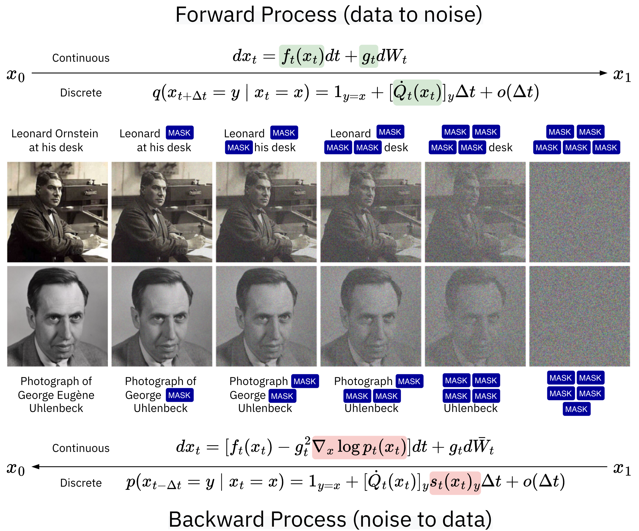
In this section, we study the score-based perspective on discrete diffusion. The main idea is to learn a transport guided by the score function $s_t(x_t)$ to reverse the diffusion process. This quantity points toward more likely samples at noise level $t$, guiding the generation process back toward the data distribution. In continuous-space diffusion models, the generation process, i.e. the backward process, is defined by the reverse SDE (see Figure 1, bottom); critically, the reverse SDE involves the score, namely $\nabla_x \log p_t(x_t)$, where $p_t$ is the distribution of the variables $x_t$ defined by the forward process.

We follow the same approach in discrete space. Since there is no SDE involved here, we work with the first-order expansion of $q(x_{t+\Delta t} | x_t)$ as $\Delta t \to 0$, which plays the role of $dx_t$ in the forward SDE, i.e. describing the evolution of $x_t$ during the corruption process. Then we reverse the process to obtain $p(x_{t-\Delta t} | x_t)$ and identify the concrete score $s_t(x_t)_{y}$, the discrete analogue of $\nabla_x \log p_t(x_t)$ (the score function of the continuous process). Finally, we learn a neural network to predict the concrete score and use it to generate new discrete data.

Forward process

In continuous-space score-based diffusion, we model the forward process as the solution of the SDE $dx_t = f_t(x_t)\,dt + g_t\,dW_t$, where we fix the drift $f_t$ and the diffusion coefficient $g_t$, and $W_t$ is a Wiener process. We follow a similar approach in discrete space: we model the forward process as a continuous-time Markov chain (CTMC), which can be written as

where we choose the forward rate matrix $\dot{Q}_t \in \mathbb{R}^{|\mathcal{V}| \times |\mathcal{V}|}$. In the above equation and in what follows, $[\dot{Q}_t(x_t)]_y$ denotes the entry of $\dot{Q}_t$ at row $x_t$ and column $y$.

For continuous-space diffusion models, the forward SDE means that over an infinitesimal time $dt$, a particle at $x_t$ moves by a deterministic drift $f_t(x_t)\,dt$ plus an independent Gaussian increment of standard deviation $g_t\sqrt{dt}$. Here, $[\dot{Q}_t(x_t)]_y$ is the instantaneous rate at which a particle at state $x_t$ jumps to state $y$: over a small interval $\Delta t$, the probability of such a jump is $[\dot{Q}_t(x_t)]_y\Delta t$ to first order.

Then, we need to specify the forward rate matrix $\dot{Q}_t$ that governs the masking process. A simple choice is to set the rate of transition from any unmasked token to the mask state:

$$\begin{equation} \htmlData{equation-label=eq:q-dot-def}{\htmlId{eq:q-dot-def}{}} \dot{Q}_t = \sigma(t) (\mathbf{1}\mathbf{e}_m^\top - I) = \sigma(t) \begin{pmatrix} -1 & 0 & \dots & 0 & 1 \\ 0 & -1 & \dots & 0 & 1 \\ \vdots & \vdots & \ddots & \vdots & \vdots \\ 0 & 0 & \dots & -1 & 1 \\ 0 & 0 & \dots & 0 & 0 \end{pmatrix}, \end{equation}$$

where $\sigma(t) > 0$ is the instantaneous masking rate, $\mathbf{e}_m$ is the one-hot vector for the mask token. The last column of $\dot{Q}_t$ indicates that the rates for jumping to $m$ are equal to $\sigma(t)$ for any token $x_t\in\mathcal{V}\setminus\{m\}$, and the last row indicates that the rate for jumping from $m$ to any other state is 0 (the mask is an absorbing state).

Continuous-space diffusion models benefits from simulation-free forward processes, which mean we can directly sample $x_t$ given $x_0$ without having to simulate the process step by step, simply using the closed-form expression $q(x_t | x_0) = \mathcal{N}\!\left(x_t;\ \sqrt{\alpha_t}\,x_0,\ (1-\alpha_t)I\right)$, where $\alpha_t = \exp\!\left(-\int_0^t \beta(s)\,ds\right)$ is the cumulative noise schedule. The same thing is possible in discrete space, we can define the transition matrix from time $0$ to time $t$, denoted $\bar{Q}_{t|0}$, such that $q(x_t | x_0)=\mathrm{Cat}(x_t;\ \bar{Q}_{t|0}^\top x_0)$. Denoting $\alpha_t = \exp\!\left(-\int_0^t \sigma(s)\,ds\right)$ the cumulative masking schedule, we have that $\bar{Q}_{t|0}$ takes the following form:

$$\begin{align} \bar{Q}_{t|0} &= \alpha_t I + (1-\alpha_t)\mathbf{1}\mathbf{e}_m^\top \\ &= \begin{pmatrix} \alpha_t & 0 & \dots & 0 & 1-\alpha_t \\ 0 & \alpha_t & \dots & 0 & 1-\alpha_t \\ \vdots & \vdots & \ddots & \vdots & \vdots \\ 0 & 0 & \dots & \alpha_t & 1-\alpha_t \\ 0 & 0 & \dots & 0 & 1 \end{pmatrix}, \htmlData{equation-label=eq:integrated-forward-transition}{\htmlId{eq:integrated-forward-transition}{}} \end{align}$$

Therefore, for a clean token $x_0$, the forward marginal is simply:

$$\begin{equation} \htmlData{equation-label=eq:ctmc-forward-marginal}{\htmlId{eq:ctmc-forward-marginal}{}} x_t = \begin{cases} x_0, & \text{with probability } \alpha_t, \\ m, & \text{with probability } 1-\alpha_t. \end{cases} \end{equation}$$

Justification of $\bar{Q}_{t|0}$

Start by composing local transitions over a partition $0=t_0<t_1<\dots<t_n=t$:

$$\begin{align} q(x_t | x_0) &= \sum_{x_{t_1},\dots,x_{t_{n-1}}} \prod_{i=0}^{n-1} q(x_{t_{i+1}} | x_{t_i}) \\ &= \left[\left(\bar{Q}_{t_1|t_0}\bar{Q}_{t_2|t_1}\cdots \bar{Q}_{t_n|t_{n-1}}\right)^\top x_0\right]_{x_t}. \end{align}$$

In the continuous-time limit, each local transition is $\bar{Q}_{t+\Delta t|t}=I+\dot{Q}_t\Delta t+o(\Delta t)$, so this product becomes the exponential of the accumulated local rates. Let $A = \mathbf{1}\mathbf{e}_m^\top - I$. Since $\dot{Q}_t = \sigma(t)A$ has a fixed matrix direction for all $t$, this integration reduces to an ordinary matrix exponential:

$$\begin{align} \bar{Q}_{t|0} &= \exp\!\left(\int_0^t \dot{Q}_s\,ds\right) \\ &= \exp\!\left(\left(\int_0^t \sigma(s)\,ds\right)A\right) \\ &= \exp(-\Lambda_t)I + \left(1-\exp(-\Lambda_t)\right)\mathbf{1}\mathbf{e}_m^\top, \end{align}$$

where $\Lambda_t = \int_0^t \sigma(s)\,ds$, hence $\alpha_t = \exp(-\Lambda_t)$.

Masked Diffusion: Forward Process

▶ forward◀ reverse

α_t =

1−t1−t²cos(tπ/2)

Startt = 0.00

T

seed

← Prev▶ PlayNext →Reset🎲 New seed

slowfast

Show N trajectories

Reverse process

In the previous section, we have described the forward process of score-based discrete diffusion models. To generate new data samples, we need to reverse the forward process.

Similarly to continuous-space diffusion, where the reverse process is obtained by reversing the forward SDE, in discrete space, the reverse process is obtained by reversing the forward Markov chain, and is also a continuous-time Markov chain.

Proof

Using Bayes’ theorem, for $y \neq x_t$:

$$\begin{align} p(x_{t-\Delta t} = y | x_t) &= \frac{q(x_t | x_{t-\Delta t} = y) q(x_{t-\Delta t} = y)}{q(x_t)} \htmlData{equation-label=eq:reverse-rate-proof-1}{\htmlId{eq:reverse-rate-proof-1}{}} \\ &= \frac{\big([\dot{Q}_t(y)]_{x_t}\Delta t + o(\Delta t)\big) \big(q(X_t = y) + O(\Delta t)\big)}{q(X_t = x_t)} \htmlData{equation-label=eq:reverse-rate-proof-2}{\htmlId{eq:reverse-rate-proof-2}{}} \\ &= \left( [\dot{Q}_t(y)]_{x_t} \frac{q(X_t = y)}{q(X_t = x_t)} \right)\Delta t + o(\Delta t) \htmlData{equation-label=eq:reverse-rate-proof-3}{\htmlId{eq:reverse-rate-proof-3}{}} \end{align}$$

By identifying this result with the definition of the reverse local transition $p(x_{t-\Delta t} = y | x_t) = \Delta t [\dot{R}_t(x_t)]_y + o(\Delta t)$, we conclude for $y \neq x_t$. For $y = x_t$, we use the fact that probabilities sum to one, so the rows of a valid transition rate matrix must sum to zero, leading to $[\dot{R}_t(x_t)]_{x_t} = - \sum_{y' \neq x_t} [\dot{R}_t(x_t)]_{y'}$.

In continuous-space diffusion, the score function $\nabla_x \log p_t(x_t)$ governs the reverse SDE, i.e. the generative process. In the discrete space, the analog to the score function is the concrete score $s_t(x_t)_y$, defined as the ratio of marginal probabilities between a candidate destination state and the current state:

$$s_t(x_t)_y \;=\; \frac{q(X_t = y)}{q(X_t = x_t)} \quad (y \neq x_t).$$

Recalling Eq. (?), the concrete score is precisely the quantity that converts the (known) forward rate $\dot{Q}_t$ into the reverse rate $\dot{R}_t$:

$$\begin{equation} \htmlData{equation-label=eq:concrete-score}{\htmlId{eq:concrete-score}{}} s_t(x_t)_y \;=\; \frac{[\dot{R}_t(x_t)]_y}{[\dot{Q}_t(x_t)]_y}. \end{equation}$$

Then the reverse process can be simulated using the concrete score as follows:

$$\begin{align} \htmlData{equation-label=eq:score-sampling}{\htmlId{eq:score-sampling}{}} x_{t-h} &\sim \mathrm{Cat}\left( \mathbf{e}_{x_t} + h\,\dot{R}_t(x_t) + o(h) \right) \\ &= \mathrm{Cat}\left( \mathbf{e}_{x_t} + h\,\big([\dot{Q}_t(x_t)]_{\cdot}\odot s_t(x_t)_{\cdot}\big) + o(h) \right), \htmlData{equation-label=eq:score-sampling-cat}{\htmlId{eq:score-sampling-cat}{}} \end{align}$$

where $\odot$ denotes the elementwise product. The forward rate $\dot{Q}_t$ is known because it is a design choice of the noising process. However, the concrete score $s_t(x_t)_y$ (or equivalently the reverse rate $\dot{R}_t$) depends on the noisy-data marginals $q(X_t=\cdot)$ which are unknown and untractable. This is why, in practice, we learn a neural approximation of it, denoted by $s_{\theta, t}(x_t)_y$.

See the reverse process conditioned on $x_0$, where the unknown $s_t(x_t)$ is replaced by the known $s_t(x_t | x_0)$ in Figure 5 by clicking the reverse button.

Training

In the forward and reverse process sections, we showed how these processes can be simulated with respectively the forward rate $\dot{Q}_t$ Eq. (?) and the reverse rate $\dot{R}_t$ Eq. (?), and that the unknown quantity connecting them is the concrete score $s_t(x_t)_y$ Eq. (?). However, this last is untractable and therefore we need to rewrite it before approximating it with a neural network $s_{\theta,t}$. To do so, we apply the marginalisation trick, meaning we express the concrete score $s_t(x_t)_y$ as a conditional expectation of the conditional concrete score $s_t(x_t | x_0)_y$ over $x_0$:

$$\begin{align} s_t(x_t)_y \;=\; \frac{p_t(y)}{p_t(x_t)} &\;=\; \frac{\sum_{x_0} p_t(y|x_0)\,p(x_0)}{p_t(x_t)} \htmlData{equation-label=eq:concrete-score-cond-exp-1}{\htmlId{eq:concrete-score-cond-exp-1}{}} \\ &\;=\; \sum_{x_0} \frac{p_t(y|x_0)}{p_t(x_t|x_0)}\; \underbrace{\frac{p_t(x_t|x_0)\,p(x_0)}{p_t(x_t)}}_{q(x_0 | x_t)\ \text{by Bayes}} \htmlData{equation-label=eq:concrete-score-cond-exp-2}{\htmlId{eq:concrete-score-cond-exp-2}{}} \\ &\;=\; \mathbb{E}_{x_0 \sim q(\cdot|x_t)}\!\left[\,s_t(x_t|x_0)_y\,\right] \htmlData{equation-label=eq:concrete-score-cond-exp-3}{\htmlId{eq:concrete-score-cond-exp-3}{}} \end{align}$$

This gives the characterization:

$$\begin{equation} \htmlData{equation-label=eq:score-kl-argmin}{\htmlId{eq:score-kl-argmin}{}} s_t \;=\; \underset{s}{\operatorname{argmin}}\ \mathbb{E}_{\substack{x_0 \sim p_0 \\ x_t \sim q(\cdot|x_0)}}\!\Bigg[ \sum_{y \neq x_t} \mathrm{KL}\!\left(s_t(x_t | x_0)_y,\, s(x_t)_y\right) \Bigg] \end{equation}$$

By weighting each term by the forward rate $[\dot{Q}_t(x_t)]_y$ (which leaves the minimizer unchanged), we can derived a new loss function to train the concrete score approximation $s_{\theta,t}$:

$$\begin{equation} \htmlData{equation-label=eq:score-kl-loss}{\htmlId{eq:score-kl-loss}{}} L_t(\theta) = \mathbb{E}_{\substack{x_0 \sim p_0 \\ x_t \sim q(\cdot|x_0)}} \Bigg[ \sum_{y \neq x_t} [\dot{Q}_t(x_t)]_y\, \mathrm{KL}\!\left(s_t(x_t | x_0)_y,\, s_{\theta,t}(x_t)_y\right) \Bigg] \end{equation}$$

Finally, by expanding the KL divergence and dropping $\theta$-independent terms, we obtain an explicit form for the score-based discrete diffusion loss:

To wrap up, we end this section with a table summarizing the important steps in score-based diffusion, put in parallel with their equivalent for continuous-space diffusion.

Table 6: Continuous-space and masked discrete score-based diffusion side by side.

Continuous-space diffusion	Masked discrete diffusion
1. Forward noising equation
$dX_t = f_t(X_t)\,dt + g_t\,dW_t$	$x_{t+\Delta t} \sim \mathrm{Cat}\!\left(\mathbf{e}_{x_t} + \dot{Q}_t(x_t)\Delta t + o(\Delta t)\right)$
2. Simulation-free forward process
$q(x_t | x_0) = \mathcal{N}\!\left(\sqrt{\alpha_t}\,x_0,\; (1-\alpha_t)I\right)$	$q(x_t | x_0) = \mathrm{Cat}\!\left(x_t;\, \alpha_t\mathbf{e}_{x_0} + (1-\alpha_t)\mathbf{e}_m\right)$
3. Reverse sampling equation
$dX_t = \left(f_t(X_t) - g_t^2 \nabla \log p_{\theta,t}(X_t)\right)dt + g_t\,d\bar{W}_t$	$x_{t-\Delta t} \sim \mathrm{Cat}\!\left(x_{t-\Delta t};\, \mathbf{e}_{x_t} + \Delta t\, \dot{R}_{\theta,t}(x_t) + o(\Delta t)\right)$
4. Concrete score
$s_{\theta,t}(x_t) = \nabla \log p_{\theta,t}(x_t) = -\dfrac{\varepsilon_{\theta,t}(x_t)}{\sqrt{1-\alpha_t}}$	$s_{\theta,t}(x_t)_y = \dfrac{p_{\theta,t}(y)}{p_{\theta,t}(x_t)} = \dfrac{[\dot{R}_{\theta,t}(x_t)]_y}{[\dot{Q}_t(x_t)]_y}$
5. Training loss (score matching)
$\mathcal{L} = \dfrac{g_t^2}{2}\,\left\| s_{\theta,t}(x_t) - \nabla \log p_t(x_t | x_0) \right\|^2$	$\mathcal{L} = \dot{Q}_t(x_t)\, \mathrm{KL}\!\left(s_t(x_t | x_0),\, s_{\theta,t}(x_t)\right)$

Equivalence between viewpoints

In the previous sections, we introduced two discrete diffusion perspectives for transporting an initial distribution to a target discrete distribution: the variational formulation and the score-based formulation. In all this section, we assume the fully corrupted distribution is $\delta_{m\ldots m}$ We will show with this assumption that these two viewpoints are equivalent, and then we connect them to discrete flow matching.

Equivalence between the two discrete diffusion perspectives

In this section, we demonstrate that variational inference and score matching viewpoints for discrete diffusion are equivalent. We first show that their sampling schemes coincide, and then that their training objectives are equivalent.

Sampling: We first connect the two views of discrete diffusion at the sampling level. The key idea is that the reverse rate $\dot{R}_t$ for score-based discrete diffusion can be written in terms of the denoiser $D_t^i(\mathbf{x})_v=\mathbb{P}(X_0^i=v | \mathbf{X}_t=\mathbf{x})$:

$$\begin{equation} \htmlData{equation-label=eq:denoiser-reverse-rate}{\htmlId{eq:denoiser-reverse-rate}{}} \dot{R}_t^i(\mathbf{x})_v = \mathbb{I}(x^i=m)\, \frac{-\dot{\alpha}_t}{1-\alpha_t} \left( D_t^i(\mathbf{x})_v - \mathbb{I}(v=m) \right). \end{equation}$$

Proof

For $s=t-h$ and a masked token $x^i=m$, Eq. (?) gives:

$$\begin{align} \mathbb{P}(X_{t-h}^i=v | \mathbf{X}_t=\mathbf{x}) &= \frac{\alpha_{t-h}-\alpha_t}{1-\alpha_t}D_t^i(\mathbf{x})_v + \frac{1-\alpha_{t-h}}{1-\alpha_t}\mathbb{I}(v=m). \htmlData{equation-label=eq:denoiser-reverse-rate-proof-1}{\htmlId{eq:denoiser-reverse-rate-proof-1}{}} \end{align}$$

Since $\alpha_{t-h}-\alpha_t=-h\dot{\alpha}_t+o(h)$, we also have $1-\alpha_{t-h}=1-\alpha_t+h\dot{\alpha}_t+o(h)$. Therefore:

$$\begin{align} \mathbb{P}(X_{t-h}^i=v | \mathbf{X}_t=\mathbf{x}) &= \mathbb{I}(v=m) + h\frac{-\dot{\alpha}_t}{1-\alpha_t} \left(D_t^i(\mathbf{x})_v-\mathbb{I}(v=m)\right) +o(h). \htmlData{equation-label=eq:denoiser-reverse-rate-proof-2}{\htmlId{eq:denoiser-reverse-rate-proof-2}{}} \end{align}$$

Comparing with the continuous-time reverse-rate definition:

$$\begin{equation} \mathbb{P}(X_{t-h}^i=v | \mathbf{X}_t=\mathbf{x}) = \mathbb{I}(v=x^i)+h\dot{R}_t^i(\mathbf{x})_v+o(h), \htmlData{equation-label=eq:denoiser-reverse-rate-proof-3}{\htmlId{eq:denoiser-reverse-rate-proof-3}{}} \end{equation}$$

and using $x^i=m$ gives Eq. (?). If $x^i\neq m$, the token is already unmasked and the reverse masked process leaves it fixed, so the rate is zero; this gives the prefactor $\mathbb{I}(x^i=m)$.

It remains to connect Eq. (?) and Eq. (?). Starting from Eq. (?), taking $s=t-h$ and letting $h \to 0$, for a masked token $x_t^i=m$:

$$\begin{align} x_{t-h}^i &\sim \mathrm{Cat}\left( \frac{\alpha_{t-h}-\alpha_t}{1-\alpha_t}D_t^i(\mathbf{x}_t) + \frac{1-\alpha_{t-h}}{1-\alpha_t}\mathbf{e}_m \right) \htmlData{equation-label=eq:masked-denoiser-euler-1}{\htmlId{eq:masked-denoiser-euler-1}{}} \\ &= \mathrm{Cat}\left( \frac{-h\dot{\alpha}_t + o(h)}{1-\alpha_t}D_t^i(\mathbf{x}_t) + \frac{1-\alpha_t + h\dot{\alpha}_t + o(h)}{1-\alpha_t}\mathbf{e}_m \right) \htmlData{equation-label=eq:masked-denoiser-euler-2}{\htmlId{eq:masked-denoiser-euler-2}{}} \\ &= \mathrm{Cat}\left( \mathbf{e}_m + h\,\frac{-\dot{\alpha}_t}{1-\alpha_t} \underbrace{\left(D_t^i(\mathbf{x}_t)-\mathbf{e}_m\right)}_{ \frac{1-\alpha_t}{-\dot{\alpha}_t}\dot{R}_t^i(\mathbf{x}_t) } + o(h) \right) \htmlData{equation-label=eq:masked-denoiser-euler-3}{\htmlId{eq:masked-denoiser-euler-3}{}} \\ &= \mathrm{Cat}\left( \mathbf{e}_{x_t^i} + h\,\dot{R}_t^i(\mathbf{x}_t) + o(h) \right). \htmlData{equation-label=eq:masked-denoiser-euler-4}{\htmlId{eq:masked-denoiser-euler-4}{}} \end{align}$$

using $\alpha_{t-h} - \alpha_t = -h\dot{\alpha}_t + o(h)$ in the second line and Eq. (?) in the third line. If $x_t^i\neq m$, both sampling processes keep the token fixed, i.e., once denoised, a token cannot be masked again or change token value.

Training Objectives: Now we turn to the corresponding training objectives. The variational perspective gives the ELBO loss Eq. (?) (which can be rewritten as Eq. (?) for Masked Diffusion), while the score-based perspective gives the concrete score matching loss Eq. (?). We now show that these two objectives are in fact the same: taking the continuous-time limit of the ELBO produces, after a change of variable, exactly the concrete score matching loss Eq. (?).

Starting from the variational loss Eq. (?), in the continuous-time limit $T \to \infty$, each discrete transition $q(x_s | x_t)$ is replaced by an instantaneous rate $\dot{R}_t(x_t)$. This motivates introducing the conditional reverse rate $\dot{R}_t(x_t | x_0)$, defined by the first-order Taylor expansion:

$$\begin{equation} \htmlData{equation-label=eq:reverse-kernel}{\htmlId{eq:reverse-kernel}{}} q(y | x_t, x_0) = \mathbb{I}(y = x_t) + \Delta t\, [\dot{R}_t(x_t | x_0)]_y + o(\Delta t), \quad y \in \mathcal{V} \end{equation}$$

For Masked Diffusion, this conditional reverse rate takes the explicit form (proof below in the spoiler):

$$\begin{equation} \htmlData{equation-label=eq:reverse-kernel-mask}{\htmlId{eq:reverse-kernel-mask}{}} \dot{R}_t(x_t | x_0) = \begin{pmatrix} & & & 0 \\ & \mathbf{0}_{|\mathcal{V}|} & & \vdots \\ & & & 0 \\ 0 & \dots \, r_t \, \dots & 0 & -r_t \end{pmatrix} = r_t\, \mathbf{e}_m (\mathbf{e}_{x_0} - \mathbf{e}_m)^\top \end{equation}$$

where $r_t = -\dot{\alpha}_t / (1 - \alpha_t)$ is the instantaneous unmasking rate, and the entry $r_t$ in the last row appears at the column index corresponding to $x_0$. Intuitively, this rate captures the instantaneous tendency of a masked token to revert to the clean token $x_0$.

Construction of $\dot{R}_t(x_t | x_0)$

To derive $\dot{R}_t(x_t | x_0)$, we write the reverse transition probabilities $q(x_s | x_t, x_0)$ for arbitrary $s < t$ using a matrix $R_{s|t}^{x_0}$, and then write the first-order Taylor expansion as $\Delta t = t - s \to 0$ of this matrix.

Using Eq. (?), the reverse transition $q(x_s | x_t, x_0)$ can be written as a categorical distribution governed by a reverse matrix $R_{s|t}^{x_0}$:

$$\begin{equation} \htmlData{equation-label=eq:bridge-cat}{\htmlId{eq:bridge-cat}{}} q(x_s | x_t, x_0) = \mathrm{Cat}\!\left(x_s;\ (R_{s|t}^{x_0})^\top x_t\right) \end{equation}$$

and:

$$\begin{align} R_{s|t}^{x_0} = \left( \begin{array}{ccc|c} & & & 0 \\ & I_{|\mathcal{V}|} & & \vdots \\ & & & 0 \\ \hline 0 & \dots \quad \frac{\alpha_s - \alpha_t}{1 - \alpha_t} \quad \dots & 0 & \frac{1 - \alpha_s}{1 - \alpha_t} \end{array} \right) \in \mathbb{R}^{K \times K} \htmlData{equation-label=eq:bridge-matrix}{\htmlId{eq:bridge-matrix}{}} \end{align}$$

where the entry $\frac{\alpha_s - \alpha_t}{1 - \alpha_t}$ in the last row appears at the column corresponding to $x_0$, and can be compactly written as $R_{s|t}^{x_0} = I + \frac{\alpha_s - \alpha_t}{1 - \alpha_t} \mathbf{e}_m(\mathbf{e}_{x_0} - \mathbf{e}_m)^\top$.

Taking the first-order Taylor expansion (noting that $\alpha_{t - \Delta t} - \alpha_t \approx -\dot{\alpha}_t \Delta t$):

$$\begin{align} R_{t - \Delta t | t}^{x_0} &= I + \frac{-\dot{\alpha}_t \Delta t}{1 - \alpha_t} \mathbf{e}_m(\mathbf{e}_{x_0} - \mathbf{e}_m)^\top + o(\Delta t) \htmlData{equation-label=eq:bridge-rate-1}{\htmlId{eq:bridge-rate-1}{}} \\ &= I + \Delta t\, \dot{R}_t(x_t | x_0) + o(\Delta t) \htmlData{equation-label=eq:bridge-rate-2}{\htmlId{eq:bridge-rate-2}{}} \end{align}$$

which identifies the conditional reverse rate as $\dot{R}_t(x_t | x_0) = r_t\, \mathbf{e}_m(\mathbf{e}_{x_0} - \mathbf{e}_m)^\top$ with $r_t = -\dot{\alpha}_t / (1 - \alpha_t)$.

Continuous-time limit proof

We start from the full ELBO derived in Eq. (?):

The first term is independent of $\theta$, so we focus on the KL terms inside the sum. Let $\Delta t = 1/T$, $t = j/T$, and $s = (j-1)/T$. Using Eq. (?) and the learned analogue of Eq. (?), the $j$-th KL $\left[ \mathrm{KL}\!\left(q\!\left(x_{(j-1)/T} | x_{j/T}, x_0\right),\, p_\theta\!\left(x_{(j-1)/T} | x_{j/T}\right)\right) \right]$ expands over the vocabulary as:

$$\begin{align} \mathrm{KL}\left(q( \cdot | x_t, x_0) , p_\theta( \cdot | x_t)\right) &= \sum_{y \in \mathcal{V}} \underbrace{q(y | x_t, x_0)}_{\mathbb{I}(y=x_t)+\Delta t[\dot{R}_t(x_t|x_0)]_y+o(\Delta t)} \log \frac{ q(y | x_t, x_0) }{ \underbrace{p_\theta(y | x_t)}_{\mathclap{\mathbb{I}(y=x_t)+\Delta t[\dot{R}_{\theta,t}(x_t)]_y+o(\Delta t)}} } \htmlData{equation-label=eq:ratio-kl-1}{\htmlId{eq:ratio-kl-1}{}} \end{align}$$

Separating the sum into the case where the token changes ($y \neq x_t$) and stays the same ($y = x_t$):

1. For $y \neq x_t$:

$$\begin{align} & (\Delta t\, [\dot{R}_t(x_t | x_0)]_y + o(\Delta t)) \log \frac{\Delta t\, [\dot{R}_t(x_t | x_0)]_y + o(\Delta t)}{\Delta t\, [\dot{R}_{\theta,t}(x_t)]_y + o(\Delta t)} \htmlData{equation-label=eq:ratio-kl-term-1}{\htmlId{eq:ratio-kl-term-1}{}} \\ & \quad = \Delta t\, [\dot{R}_t(x_t | x_0)]_y \log \frac{[\dot{R}_t(x_t | x_0)]_y}{[\dot{R}_{\theta,t}(x_t)]_y} + o(\Delta t) \notag \end{align}$$

2. For $y = x_t$, using the expansion $\log \frac{1+a}{1+b} = a - b + o(|a|+|b|)$:

$$\begin{align} & (1 + \Delta t\, [\dot{R}_t(x_t | x_0)]_{x_t} + o(\Delta t)) \log \frac{1 + \Delta t\, [\dot{R}_t(x_t | x_0)]_{x_t} + o(\Delta t)}{1 + \Delta t\, [\dot{R}_{\theta,t}(x_t)]_{x_t} + o(\Delta t)} \htmlData{equation-label=eq:ratio-kl-term-2-1}{\htmlId{eq:ratio-kl-term-2-1}{}} \notag \\ & \quad = \Delta t\, [\dot{R}_t(x_t | x_0)]_{x_t} - \Delta t\, [\dot{R}_{\theta,t}(x_t)]_{x_t} + o(\Delta t) \htmlData{equation-label=eq:ratio-kl-term-2-2}{\htmlId{eq:ratio-kl-term-2-2}{}} \\ & \quad = \Delta t \left( - \sum_{y \neq x_t} [\dot{R}_t(x_t | x_0)]_y + \sum_{y \neq x_t} [\dot{R}_{\theta,t}(x_t)]_y \right) + o(\Delta t) \htmlData{equation-label=eq:ratio-kl-term-2-3}{\htmlId{eq:ratio-kl-term-2-3}{}} \end{align}$$

Combining these terms, the $j$-th KL term becomes:

$$\begin{align} \mathrm{KL} &= \Delta t \sum_{y \neq x_t} \Bigg( [\dot{R}_{\theta,t}(x_t)]_y - [\dot{R}_t(x_t | x_0)]_y \log [\dot{R}_{\theta,t}(x_t)]_y \htmlData{equation-label=eq:ratio-kl-sum-1}{\htmlId{eq:ratio-kl-sum-1}{}} \\ &\quad + \underbrace{ [\dot{R}_t(x_t | x_0)]_y \log [\dot{R}_t(x_t | x_0)]_y - [\dot{R}_t(x_t | x_0)]_y }_{\text{ independent of }\theta} \Bigg) + o(\Delta t). \notag \end{align}$$

Writing $t_t=j/T$ and $\Delta t=1/T$, the ELBO Eq. (?) is therefore (grouping the $\theta$-independent above and $\mathrm{KL}(q(x_1 | x_0) , p_T)$ into a constant $C$):

$$\begin{align} &\sum_{j=1}^{T} \mathbb{E}_{x_{t_t}\sim q(\cdot|x_0)} \left[ \mathrm{KL}\left(q(x_{t_t-\Delta t}|x_{t_t},x_0),p_\theta(x_{t_t-\Delta t}|x_{t_t})\right) \right] \htmlData{equation-label=eq:final-celbo}{\htmlId{eq:final-celbo}{}} \\ &= \sum_{j=1}^{T}\Delta t\, \mathbb{E}_{x_{t_t}\sim q(\cdot|x_0)} \Bigg[ \sum_{y\neq x_{t_t}} \bigg( [\dot{R}_{\theta,t_t}(x_{t_t})]_y -[\dot{R}_{t_t}(x_{t_t}|x_0)]_y \log [\dot{R}_{\theta,t_t}(x_{t_t})]_y \htmlData{equation-label=eq:ratio-riemann-1}{\htmlId{eq:ratio-riemann-1}{}} \bigg) \Bigg] + C + o(1), \notag \end{align}$$

where $C$ collects the terms independent of $\theta$. Taking $T\to\infty$ turns the sum into a Riemann integral over $t$, whose integrand is exactly the loss Eq. (?).

It remains to express Eq. (?) in terms of the concrete score. Writing the reverse rates as $[\dot{R}_{t}(x_t)]_y = [\dot{Q}_t(x_t)]_y\,s_{t}(x_t)_y$ (see Eq. (?)), we recover, up to a $\theta$-independent constant, the concrete score matching loss Eq. (?) established in the score-based perspective. The two viewpoints therefore minimize the same objective.

Equivalence derivation

Applying Bayes’ theorem to $x_t \to x_s$ conditioned on $x_0$ gives:

$$\begin{equation} \htmlData{equation-label=eq:reverse-bayes}{\htmlId{eq:reverse-bayes}{}} \dot{R}_t(x_t | x_0)_y = [\dot{Q}_t(x_t)]_y \frac{p_t(y|x_0)}{p_t(x_t|x_0)} \end{equation}$$

Substituting $[\dot{R}_{\theta,t}(x_t)]_y = [\dot{Q}_t(x_t)]_y\,s_{\theta,t}(x_t)_y$ and the expression above into Eq. (?):

$$\begin{equation} \htmlData{equation-label=eq:score-loss}{\htmlId{eq:score-loss}{}} \begin{aligned} L_t(\theta) &= \mathbb{E}_{\substack{x_0 \sim p_0 \\ x_t \sim q( \cdot |x_0)}} \Bigg[ \sum_{y \neq x_t} \Bigg( [\dot{Q}_t(x_t)]_y s_{\theta,t}(x_t)_y \\ &\quad - \left( [\dot{Q}_t(x_t)]_y \frac{p_t(y|x_0)}{p_t(x_t|x_0)} \right) \log \left( [\dot{Q}_t(x_t)]_y s_{\theta,t}(x_t)_y \right) \Bigg) \Bigg] \end{aligned} \end{equation}$$

Expanding the logarithm gives:

$$\begin{align} L_t(\theta) &= \mathbb{E}_{\substack{x_0 \sim p_0 \\ x_t \sim q( \cdot |x_0)}} \Bigg[ \sum_{y \neq x_t} \Bigg( [\dot{Q}_t(x_t)]_y s_{\theta,t}(x_t)_y \htmlData{equation-label=eq:score-loss-expand-1}{\htmlId{eq:score-loss-expand-1}{}} \\ &\qquad - [\dot{Q}_t(x_t)]_y \frac{p_t(y|x_0)}{p_t(x_t|x_0)} \log [\dot{Q}_t(x_t)]_y \notag \\ &\qquad - [\dot{Q}_t(x_t)]_y \frac{p_t(y|x_0)}{p_t(x_t|x_0)} \log s_{\theta,t}(x_t)_y \Bigg) \Bigg]. \notag \\ &= \mathbb{E}_{\substack{x_0 \sim p_0 \\ x_t \sim q( \cdot |x_0)}} \Bigg[ \sum_{y \neq x_t} [\dot{Q}_t(x_t)]_y \bigg( s_{\theta,t}(x_t)_y - \frac{p_t(y|x_0)}{p_t(x_t|x_0)} \log s_{\theta,t}(x_t)_y \bigg) \Bigg] \htmlData{equation-label=eq:score-loss-expand-group-1}{\htmlId{eq:score-loss-expand-group-1}{}} \\ &\quad + \underbrace{ \mathbb{E}_{\substack{x_0 \sim p_0 \\ x_t \sim q( \cdot |x_0)}} \Bigg[ \sum_{y \neq x_t} - [\dot{Q}_t(x_t)]_y \frac{p_t(y|x_0)}{p_t(x_t|x_0)} \log [\dot{Q}_t(x_t)]_y \Bigg] }_{C\ \text{independent of }\theta}. \notag \end{align}$$

This is exactly the loss Eq. (?) of the concrete score matching proposition.

Equivalence with discrete flow matching

We now connect discrete diffusion to discrete flow matching. In discrete flow matching, a velocity field $u_t$ defines the Euler sampling scheme:

$$\begin{equation} \htmlData{equation-label=eq:dfm-euler-sampling}{\htmlId{eq:dfm-euler-sampling}{}} x_{t+h} \sim \mathrm{Cat}\!\left(\mathbf{e}_{x_t} + h\,u_t(x_t)\right). \end{equation}$$

We show that this sampling rule is equivalent to sampling in discrete diffusion (Eq. (?)).

Sampling: To align these two sampling equations directly, we must first account for the main discrepancy between the frameworks: their time conventions. In discrete diffusion, $t = 0$ corresponds to clean data, and $t = 1$ corresponds to the fully masked state. Discrete flow matching uses the exact opposite convention.

Suppose we know the discrete diffusion reverse rate $\dot{R}_t$. We define the flow matching velocity by the time reversal:

$$\begin{equation} \htmlData{equation-label=eq:time-reversal}{\htmlId{eq:time-reversal}{}} u_{t'}^{\text{FM}} = \dot{R}_{1-t'} \end{equation}$$

Then, sampling from discrete diffusion using Eq. (?) is equivalent to sampling from the flow matching Euler scheme Eq. (?): for every $t'\in[0,1]$, the distribution $p^{\mathrm{FM}}_{t'}$ of samples obtained by simulating flow matching from $0$ to $t'$ is the same as the distribution $p^{\mathrm{DD}}_{1-t'}$ obtained by simulating the discrete diffusion reverse CTMC from $1$ to $1-t'$, i.e. $p^{\mathrm{FM}}_{t'} = p^{\mathrm{DD}}_{1-t'}$.

Proof

We start from the infinitesimal reverse-time transition of the discrete diffusion process Eq. (?).

We first perform the variable change $t' = 1 - t$ in Eq. (?). We have $t = 1 - t'$, so $x_t = x_{1-t'}$ and $x_{t - \Delta t} = x_{1 - t' - \Delta t}$. The rate evaluates at $\dot{R}_{1-t'}$, giving:

$$\begin{equation} \htmlData{equation-label=eq:time-change}{\htmlId{eq:time-change}{}} p(x_{1-t'-\Delta t} = y | x_{1-t'}) = \mathbb{I}(y = x_{1-t'}) + \Delta t \, [\dot{R}_{1-t'}(x_{1-t'})]_y + o(\Delta t) \end{equation}$$

Since $t_{\text{FM}} = 1 - t_{\text{DD}}$, we identify $x^{\text{FM}}_{t'} = x_{1-t'}$. We deduce $x^{\text{FM}}_{t' + \Delta t} = x_{1 - t' - \Delta t}$. Substituting these identities into Eq. (?):

$$\begin{equation} \htmlData{equation-label=eq:fm-step}{\htmlId{eq:fm-step}{}} p(x^{\text{FM}}_{t' + \Delta t} = y | x^{\text{FM}}_{t'}) = \mathbb{I}(y = x^{\text{FM}}_{t'}) + \Delta t \, [\dot{R}_{1-t'}(x^{\text{FM}}_{t'})]_y + o(\Delta t) \end{equation}$$

Recall the definition of a probability velocity: a velocity field $u_{t'}$ generates a process $x^{\text{FM}}_{t'}$ if and only if $p(x^{\text{FM}}_{t' + \Delta t} = y | x^{\text{FM}}_{t'} = x) = \mathbb{I}(y = x^{\text{FM}}_{t'}) + \Delta t \, [u_{t'}(x^{\text{FM}}_{t'})]_y + o(\Delta t)$.

Identifying the first-order terms in Eq. (?) with the probability-velocity definition directly gives:

$$\begin{equation} \htmlData{equation-label=eq:time-reversal-velocity}{\htmlId{eq:time-reversal-velocity}{}} [u_{t'}^{\text{FM}}(x)]_y = [\dot{R}_{1-t'}(x)]_y \end{equation}$$

and therefore $u_{t'}^{\text{FM}} = \dot{R}_{1-t'}$.

Training Objectives: Now we show how their training objectives line up. The variational diffusion perspective gives the Masked Diffusion objective Eq. (?). In discrete flow matching, the velocity can be parameterized through a denoiser $P_{\theta,t}(X_1^i = x_1^i | X_t=\mathbf{x})$, trained with the cross-entropy objective:

$$\begin{equation} \htmlData{equation-label=eq:cdm-loss}{\htmlId{eq:cdm-loss}{}} L_{\text{CDM}}(\theta) = -\mathbb{E}_{\substack{t \sim \mathcal{U}(0,1) \\ \mathbf{x}_1 \sim p_0 \\ \mathbf{x} \sim p_t( \cdot | \mathbf{x}_1)}} \left[ \sum_{i=1}^S \log P_{\theta,t}(X_1^i = x_1^i | X_t = \mathbf{x}) \right]. \end{equation}$$

To directly compare the two training losses, we first note that the denoiser used by discrete flow matching and the denoiser used by variational diffusion in Eq. (?) are exactly the same object. Applying the time reversal $t_{\text{FM}} = 1 - t_{\text{DD}}$ and identifying the clean data $x_1=x_0$, we get:

$$\begin{align} D_{\theta,t_{\text{DD}}}^i(\mathbf{x})_{x_0^i} &= P_{\theta,t_{\text{DD}}}(X_0^i=x_0^i | X_{t_{\text{DD}}}=\mathbf{x}) \htmlData{equation-label=eq:denoiser-time-identification-1}{\htmlId{eq:denoiser-time-identification-1}{}} \\ &= P_{\theta,t_{\text{FM}}}(X_1^i=x_1^i | X_{t_{\text{FM}}}=\mathbf{x}). \htmlData{equation-label=eq:denoiser-time-identification-2}{\htmlId{eq:denoiser-time-identification-2}{}} \end{align}$$

Derivation

Under the time reversal above, the weight in Eq. (?) satisfies $-\dot{\alpha}_{t_{\text{DD}}}/(1-\alpha_{t_{\text{DD}}})=1/t_{\text{DD}}=1/(1-t_{\text{FM}})$. Therefore the Masked Diffusion loss Eq. (?) becomes the weighted masked cross-entropy:

$$\begin{equation} \htmlData{equation-label=eq:mdm-mask-loss-fm-time}{\htmlId{eq:mdm-mask-loss-fm-time}{}} L_{\text{MDM}}(t) = \mathbb{E}\!\left[\,\sum_{i=1}^S \mathbb{I}(x_t^i = m) \cdot \frac{1}{1-t} \cdot \left(-\log P_{\theta,t}(X_1^i = x_1^i | \mathbf{x}_t)\right)\right]. \end{equation}$$

Since $P(x_t^i = m) = 1-t$, applying the law of total expectation, $\mathbb{E}[Z]=P(x_t^i=m)\mathbb{E}[Z|x_t^i=m]+P(x_t^i\neq m)\mathbb{E}[Z|x_t^i\neq m]$:

$$\begin{align} L_{\text{MDM}}(t) \htmlData{equation-label=eq:mdm-t-1}{\htmlId{eq:mdm-t-1}{}} &= (1-t) \cdot \frac{1}{1-t} \cdot \mathbb{E}\!\left[ \htmlData{equation-label=eq:mdm-t-2}{\htmlId{eq:mdm-t-2}{}} -\log P_{\theta,t}(X_1^i = x_1^i | \mathbf{x}_t) \htmlData{equation-label=eq:mdm-t-3}{\htmlId{eq:mdm-t-3}{}} | x_t^i = m \htmlData{equation-label=eq:mdm-t-4}{\htmlId{eq:mdm-t-4}{}} \right] \htmlData{equation-label=eq:mdm-t-5}{\htmlId{eq:mdm-t-5}{}} \\ &\quad + t \cdot \underbrace{\mathbb{E}\!\left[ \mathbb{I}(x_t^i=m)\frac{1}{1-t} \left(-\log P_{\theta,t}(X_1^i = x_1^i | \mathbf{x}_t)\right) | x_t^i \neq m \right]}_{0\ \text{since }x_t^i\neq m} \notag \\ &= \mathbb{E}\!\left[ \htmlData{equation-label=eq:mdm-t-6}{\htmlId{eq:mdm-t-6}{}} -\log P_{\theta,t}(X_1^i = x_1^i | \mathbf{x}_t) \htmlData{equation-label=eq:mdm-t-7}{\htmlId{eq:mdm-t-7}{}} | x_t^i = m \htmlData{equation-label=eq:mdm-t-8}{\htmlId{eq:mdm-t-8}{}} \right]. \htmlData{equation-label=eq:mdm-t-9}{\htmlId{eq:mdm-t-9}{}} \end{align}$$

We decompose $L_{\text{CDM}}$ using the same law of total expectation, splitting over masked and unmasked positions:

$$\begin{align} L_{\text{CDM}}(t) \htmlData{equation-label=eq:cm-t-1}{\htmlId{eq:cm-t-1}{}} &= (1-t) \cdot \mathbb{E}\!\left[ \htmlData{equation-label=eq:cm-t-2}{\htmlId{eq:cm-t-2}{}} -\log P_{\theta,t}(X_1^i = x_1^i | \mathbf{x}_t) \htmlData{equation-label=eq:cm-t-3}{\htmlId{eq:cm-t-3}{}} | x_t^i = m \htmlData{equation-label=eq:cm-t-4}{\htmlId{eq:cm-t-4}{}} \right] \htmlData{equation-label=eq:cm-t-5}{\htmlId{eq:cm-t-5}{}} \\ &\quad + t \cdot \mathbb{E}\!\left[ \htmlData{equation-label=eq:cm-t-6}{\htmlId{eq:cm-t-6}{}} -\log P_{\theta,t}(X_1^i = x_1^i | \mathbf{x}_t) \htmlData{equation-label=eq:cm-t-7}{\htmlId{eq:cm-t-7}{}} | x_t^i \neq m \htmlData{equation-label=eq:cm-t-8}{\htmlId{eq:cm-t-8}{}} \right]. \notag \end{align}$$

For unmasked positions $i$, a well trained denoiser should just copy the current token $x_t^i=x_1^i$ it sees, therefore $P_{\theta,t}(X_1^i=x_1^i|\mathbf{x}_t)=1$, and the second term vanishes, giving:

$$\begin{equation} \htmlData{equation-label=eq:cm-mask-loss}{\htmlId{eq:cm-mask-loss}{}} L_{\text{CDM}}(t) \approx (1-t) \cdot \mathbb{E}\!\left[ -\log P_{\theta,t}(X_1^i = x_1^i | \mathbf{x}_t) | x_t^i = m \right]. \end{equation}$$

Both expressions share the same conditional expectation. Eliminating it yields Eq. (?).

Disclaimer In general, learning a velocity field $u$ (or equivalently a reverse rate $\dot{R}$) with Eq. (?) is not equivalent to learning a denoiser with Eq. (?) for arbitrary source distributions or paths, for instance under uniform diffusion.

References

Notes

References

Argmax Flows and Multinomial Diffusion: Learning Categorical Distributions[PDF]
Emiel Hoogeboom, Didrik Nielsen, Priyank Jaini, Patrick Forre, Max Welling. NeurIPS 2021.
Structured Denoising Diffusion Models in Discrete State-Spaces[PDF]
Jacob Austin, Daniel D. Johnson, Jonathan Ho, Daniel Tarlow, Rianne van den Berg. NeurIPS 2021.
A Continuous Time Framework for Discrete Denoising Models[PDF]
Andrew Campbell, Joe Benton, Tom Rainforth, George Deligiannidis, Arnaud Doucet. NeurIPS 2022.
Discrete Diffusion Modeling by Estimating the Ratios of the Data Distribution[PDF]
Aaron Lou, Chenlin Meng, Stefano Ermon. ICML 2024.
Generative Flows on Discrete State-Spaces: Enabling Multimodal Flows with Applications to Protein Co-Design[PDF]
Andrew Campbell, Jason Yim, Regina Barzilay, Tom Rainforth, Tommi Jaakkola. ICML 2024.
DiGress: Discrete Denoising diffusion for graph generation[PDF]
Clement Vignac, Igor Krawczuk, Antoine Siraudin, Bohan Wang, Volkan Cevher, Pascal Frossard. ICLR 2023.
Scaling Rectified Flow Transformers for High-Resolution Image Synthesis[PDF]
Patrick Esser, Sumith Kulal, Andreas Blattmann, Rahim Entezari, Jonas Müller, Harry Saini, Yam Levi, Dominik Lorenz, Axel Sauer, Frederic Boesel, Dustin Podell, Tim Dockhorn, Zion English, Kyle Lacey, Alex Goodwin, Yannik Marek, Robin Rombach. ICML 2024.
Stable Video Diffusion: Scaling Latent Video Diffusion Models to Large Datasets[PDF]
Andreas Blattmann, Tim Dockhorn, Sumith Kulal, Daniel Mendelevitch, Maciej Kilian, Dominik Lorenz, Yam Levi, Zion English, Vikram Voleti, Adam Letts, Varun Jampani, Robin Rombach. Arxiv 2023.
Generative Modeling by Estimating Gradients of the
Data Distribution[PDF]
Yang Song, Stefano Ermon, NeurIPS 2019.
Deep Unsupervised Learning using Nonequilibrium Thermodynamics[PDF]
Jascha Sohl-Dickstein, Eric Weiss, Niru Maheswaranathan, Surya Ganguli. PMLR 2015.
Score-Based Generative Modeling through Stochastic Differential Equations[PDF]
Yang Song, Jascha Sohl-Dickstein, Diederik P. Kingma, Abhishek Kumar, Stefano Ermon, Ben Poole. ICLR 2021.
Simplified and Generalized Masked Diffusion for Discrete Data[PDF]
Jiaxin Shi, Kehang Han, Zhe Wang, Arnaud Doucet, Michalis K. Titsias. NeurIPS 2024.
Here KL denotes the generalized KL divergence between two positive vectors a,b∈R+d, KL(a,b)=∑j=1dajlog(aj/bj)−aj+bj.
Up to a constant C independent of θ, Eq. (?) is
KL(R˙t(xt∣x0),R˙θ,t(xt)).
We note q(xs∣xt,x0) the conditional law
q(Xs=⋅∣Xt=xt,X0=x0).
For simplicity, we consider [Dθ,t(xt)]m=0.
Passing from the single-token derivation to the full sequence uses two assumptions:
The forward transition factorizes token-wise:
q(Xt=xt∣Xs=xs)=∏i=1Sq(Xti=xti∣Xsi=xsi).
The denoiser factorizes position per position:
P(X0=x0∣Xt=xt)=∏i=1SP(X0i=x0i∣Xt=xt).
Each per-position prediction still use the whole current sequence xt as context.